Math functions

Visualization of mathematical functions

Make use of some numpy functions (numpy.arange) and get a feel for some vector manipulation.

Attention

Exercise 4.5:

Visualize \(f(t)=\sin(\omega t + \phi_0)\) for a given frequency \(\omega = 1.2Hz\) and phase shift \(\phi_0 = 1.0\) over the time interval \(t = 0...10\) at discrete time intervals \(dt = 0.001\) s.
Visualize \(f^2(t)\) (squared). What happens if you reduced dt to 1 s ?
Visualize a Gaussian peak:

\[f(x) = Ae^{-\frac{(x-x_0)^2}{\sigma_x}}\]

where x is the independent variable and the factors \(x_0\) , \(A\), and \(\sigma_x\) determine the shape of the function. Make sure that you understand what each parameter pertains to.

More loops

Attention

Exercise 4.6:

Visualize a 2D Gaussian peak:

\[f(x,y) = Ae^{-\frac{(x-x_0)^2}{\sigma_x}-\frac{(y-y_0)^2}{\sigma_y}}\]

using a nested for loop. This is harder. In essence you will need to fill a 2D array and visualize it with colors using plt.pcolormesh(). Then do the same but replace the nested for loops using numpys "meshgrid". What is easier?

Recursion

There is a third way to do loops in Python (and other programming languages as well): If you define a function you can call that function recursively:

def Fibonacci(n):
    if n < 0:
        raise ValueError(f"Negative numbers are not allowed: {n}")
    elif n == 0:
        return 0
    elif n == 1 or n == 2:
        return 1
    else:
        return Fibonacci(n - 1) + Fibonacci(n - 2)

print(f"F0: {Fibonacci(0)}")
print(f"F1: {Fibonacci(1)}")
print(f"F2: {Fibonacci(2)}")
print(f"F3: {Fibonacci(3)}")
print(f"F9: {Fibonacci(9)}")

Mathematically the Fibonacci numbers are defined as:

\[\begin{split}F_{n} = \left\{ \begin{array}{ll} 0, & n = 0 \\ 1, & n = 1 \\ F_{n-1} + F_{n-2}, & n > 1 \end{array} \right.\end{split}\]

Attention

Exercise 4.7:

Now write the Fibonacci function in a non-recursive way using a for loop or a while loop.

Regressions

Regression analysis is a way to determine a realtion between different parameters or variables. Such a relation might be linear (first order) or polynominal (higher order). To determine how good the fit of the regression is to the actual data, we can calcualte the \(R^2\) value. The higher the \(R^2\) value, the better the fit to the data. Let’s look at the figure below. Here the green dots are our exemplary datapoint. Panel 1 shows a linear fit, Panel 2 a second order, Panel 3 a third order and Panel 4 a forth order fit. We see the \(R^2\) value increasing with every panel. In this example the exemplary data is created using a forth order polynominal function.

Using the polyfit function you can fit a n-th order function to your data. The output of this function then is a vector of coefficients p that minimise the squared error of the fit to the data. For instance for a linear fit the fit looks like:

\[y(x) = mx + b\]

for a 2nd-5th order polynominal:

\[ \begin{align}\begin{aligned}y(x) = ax^2 + bx + c\\y(x) = ax^3 + bx^2 + cx + d\\y(x) = ax^4 + bx^3 + cx^2 + dx + e\\y(x) = ax^5 + bx^4 + cx^3 + dx^2 + ex + f\end{aligned}\end{align} \]

To evalualte this polynominal at specific values (given as x) use the polyval function.

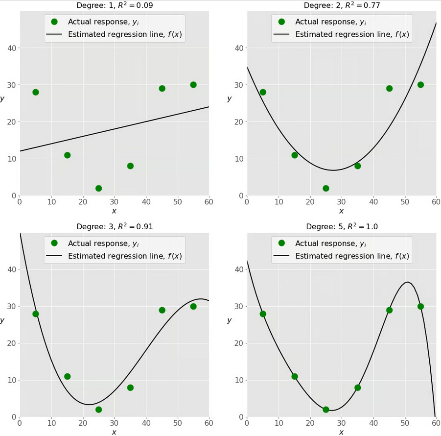
You can read more about it here: https://en.wikipedia.org/wiki/Coefficient_of_determination

Attention

Exercise 4.8:

Load the Keeling curve. Fit a first and second order polynomial to the dataset. We understand that this type of fitting must have been solved by somebody else already and therefore use functions to do the task, specifically numpy’s polyfit and polyval combination. Visualize the seasonality by subtracting the fit from the observations. Which models (i.e. first or second order polynomial) fits better and what does that mean?